基于 Delaunay 三角剖分的 FSAE 路径规划算法
本文最后更新于 2023年3月6日 下午
本文为项目 FSAE-PathPlanning-Delaunay 之文档,完整代码见 https://github.com/muziing/FSAE-PathPlanning-Delaunay
引言
在 FSAE(大学生方程式赛车)无人车比赛中,赛车需要根据传感器返回的作为路径边界标识的交通锥桶的信息(颜色、位置坐标),进行路径规划,进而为下一刻的控制提供依据。良好的路径规划算法应能够根据离散的锥桶坐标,快速规划出一条光滑、连续、合理靠近车道中心线的目标路径。
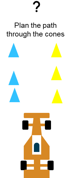
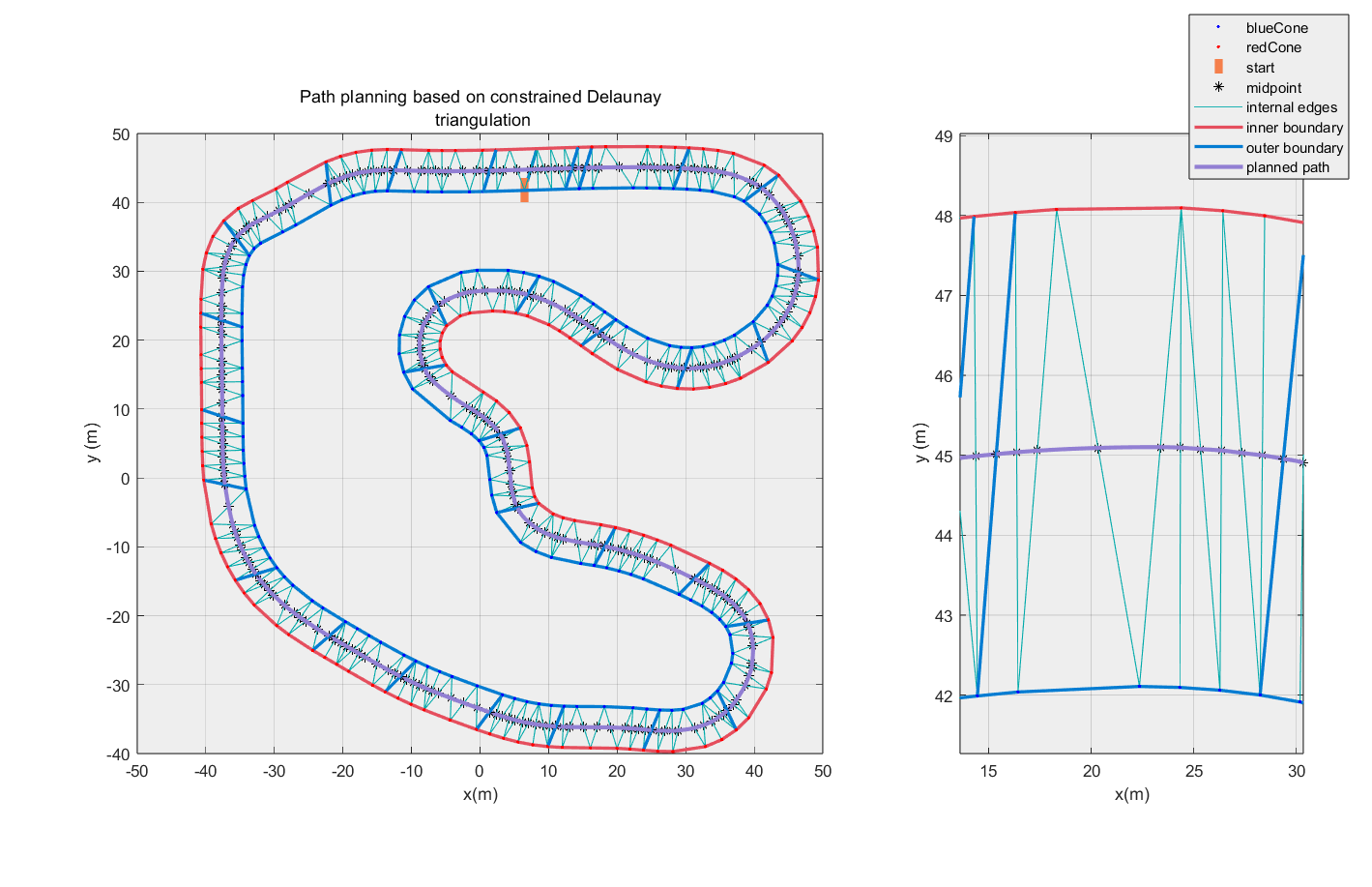
本文介绍了一种基于 Delaunay 三角剖分的路径规划算法:将锥桶位置视为离散点,构建 Delaunay 三角,然后以位于车道内部的那些三角形边的中点为依据进行插值,最终得到期望路径。经验证,该算法基本可以完成路径规划任务。
背景知识:Delaunay三角剖分
创建Delaunay三角剖分
读取加载数据
首先从 CSV 文件中导入锥桶位置坐标。
CSV 数据示例如下,
1 | |
- 第一列为锥桶序号,内外侧锥桶已经分别按照赛道顺序排序
- 第二列为锥桶类型(颜色),
2为外侧锥桶(蓝色,位于车辆行驶方向的左侧)、11为内侧锥桶(黄色,位于车辆行驶方向的右侧) - 第三四列为 x 坐标与 y 坐标,单位为 [m]
编写 MATLAB 代码读取数据:
1 | |
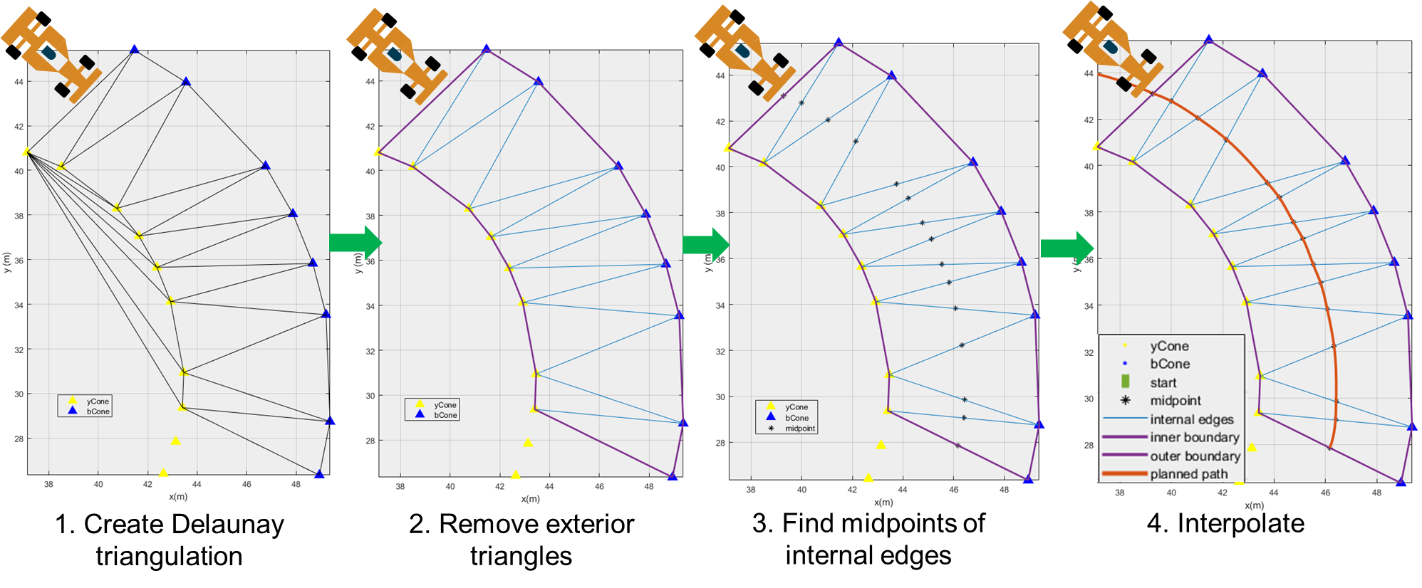
此时已将内、外侧锥桶的xy位置坐标分别存储在 innerConePosition 与 outerConePosition 两张 table 中。
数据预处理
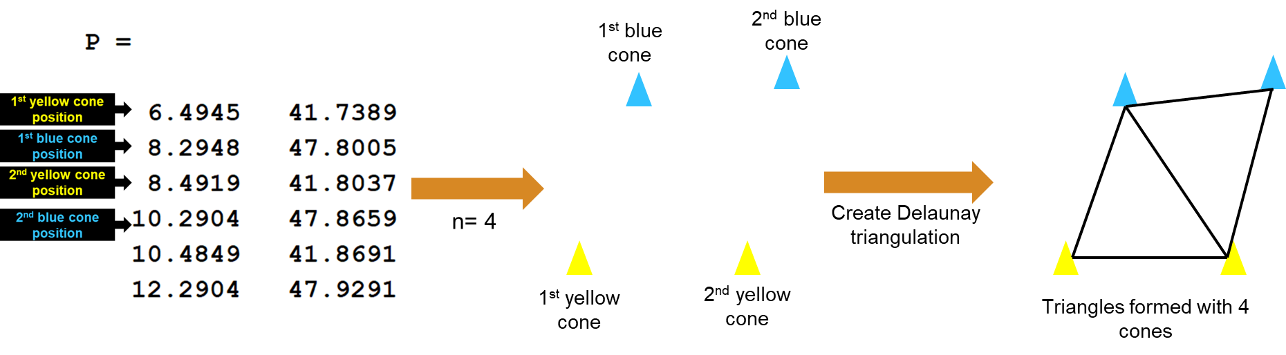
然后需要将内外侧锥桶的坐标交替合并,得到将用于创建 delaunayTriangulation 对象的 P 矩阵。
1 | |
在真实场景中,安装在赛车上的传感器的感知范围是有限的,并不能一次获取所有锥桶位置。因此,设计一个变量 interval,用于控制每次规划时考虑的锥桶数量。(换言之,将整条赛道划分为若干个路段,每次只在一个路段内进行规划。)如图所示,若 interval = 4,则将基于每 4 个锥桶坐标创建 Delaunay 三角剖分。
1 | |
构建三角形
用一个 for 循环控制,每次循环中进行一个路段的路径规划,循环完成后即完成整条赛道的路径规划。注意此段之后代码的缩进,表明后续代码均在此循环体内:
1 | |
计算出属于该路段的坐标点集索引 pointIndex,P(pointIndex, :) 即为属于该路段的坐标。以此创建 delaunayTriangulation 对象 delaTria。
1 | |
Delaunay 三角剖分可视化:
1 | |

移除外部三角形
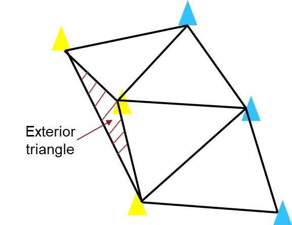
如图所示,在进行三角剖分时,可能会创建出落在赛道之外的三角形,进而导致后续产生错误的路径。因此需要通过施加约束边界 C 去除这些外部三角形。
定义约束
约束边界 C 是一个由约束边的顶点 ID 所组成的两列矩阵,它的每一行对应一条约束边,其中:
C(j, 1)为第 j 条约束边起始顶点的 IDC(j, 2)为第 j 条约束边末端顶点的 ID
下图显示了由矩阵 C = [2 1;1 3;3 5;5 6;2 4;4 6] 所定义的约束边界。

通过如下代码生成约束边界矩阵 C:
1 | |
创建带有约束的 Delaunay 三角剖分
定义约束后,使用 delaunayTriangulation 对象创建二维 Delaunay 三角剖分:
1 | |
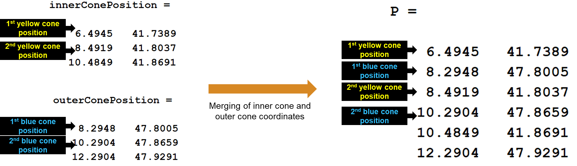
在继续下一步之前,需要介绍一下 delaunayTriangulation 的 Connectivity List(连接列表)属性。该属性将在后续步骤中被使用,实现通过排除外部三角形来创建新的三角剖分。
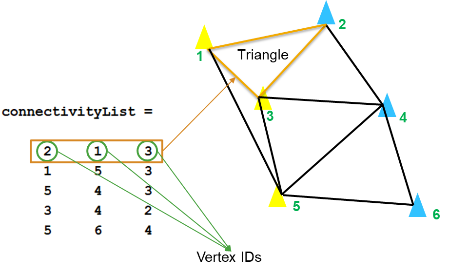
根据文档,一个三角剖分(如 DT)的连接列表是一个具有以下特征的矩阵:
DT.ConnectivityList中的每个元素是一个顶点 ID- 每一行中的顶点构成了三角剖分中的一个三角形
- 行号对应于该行所表示的一个三角形 的ID
例如,在下图中,第一行的 [2 1 3] 表示三角剖分后产生的第一个三角形。
在了解连接列表的含义之后,让我们看看如何利用带约束的 Delaunay 三角剖分 TR 的连接表来移除外部三角形。
1 | |
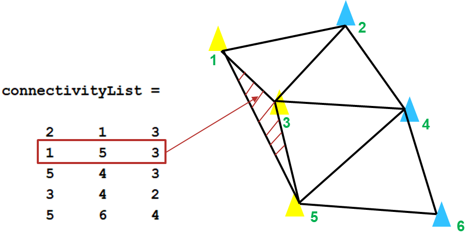
获得连接矩阵 TRC 后,要删除构成外部三角形的那些行。如下图示意,第二行 [1 5 3] 代表的是一个外部三角形。
调用 delaunayTriangulation 对象的函数,可以实现各种拓扑与几何查询。在此处使用对象函数 isInterior 来检查每一行 ID 的三角形是否在有界几何区域内。该函数返回一个由逻辑值(布尔值)所组成的列向量:如果第 n 个逻辑值为 true,则三角剖分中的第 n 个三角形在约束区域 C 内,否则该三角形在约束区域 C 外,为外部三角形。

1 | |
通过上述处理,获得了不包含外部三角形的新的连接列表矩阵 TC。然后依据 TC,从 delaTriaPoints 包含的点中创建一个新的二维三角剖分:
1 | |
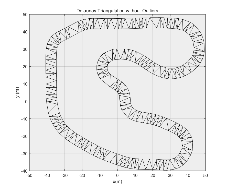
绘图,可视化观察可知,已经成功去除了外部三角形。
1 | |
获取中点与平滑处理
获取内部边中点
如下图所示,寻找所有位于车道内部的三角形边的中点,连接这些中点即为初步规划出的路径:
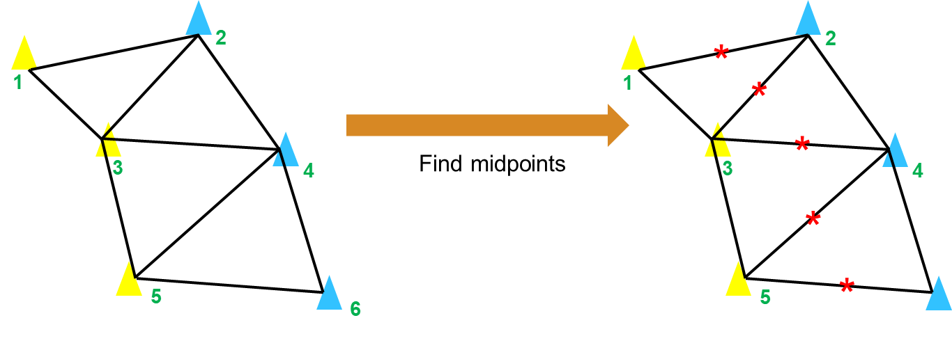
1 | |
中心点插值
最后,为了使获得的路径足够光滑,还需要在中心点之间进行插值,插值点的数量由变量 interpolationNum 控制:
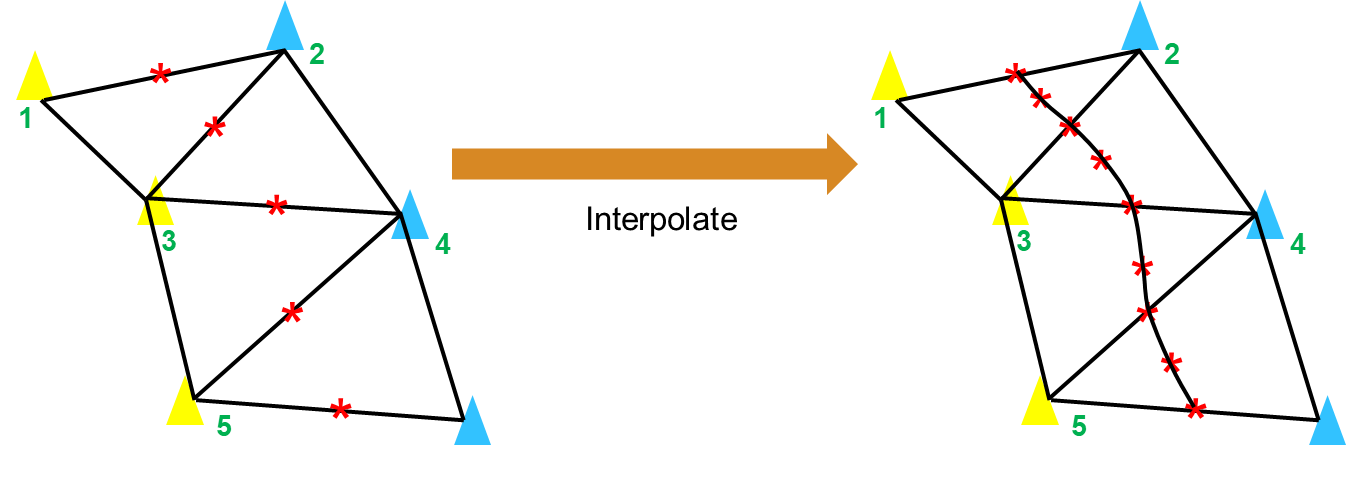
1 | |
期望路径可视化
对最终规划结果进行可视化:
1 | |
其中 pathPlanPlot() 函数代码如下:
1 | |