基于OpenCV的交通信号灯识别
本文最后更新于 2023年1月10日 晚上
简介
本文介绍了一种用于交通信号灯图像识别分类的算法:使用 OpenCV-Python,通过将图像转换至 HSV 色彩空间,使得其中的颜色更容易被分割,达到识别分类目的。仅运用图像处理方法,而没有使用机器学习方法。经简单调参,在测试集上可以达到98%以上的准确率。
本项目 fork 自shawshany/traffic_light_classified,保留其算法思想。做删去冗余部分,重写大部分代码,添加大量docstring,增强可扩展性与鲁棒性等处理。
本文算法代码与图像集已全部开源至Github - muziing/Traffic-Lights-Classification。
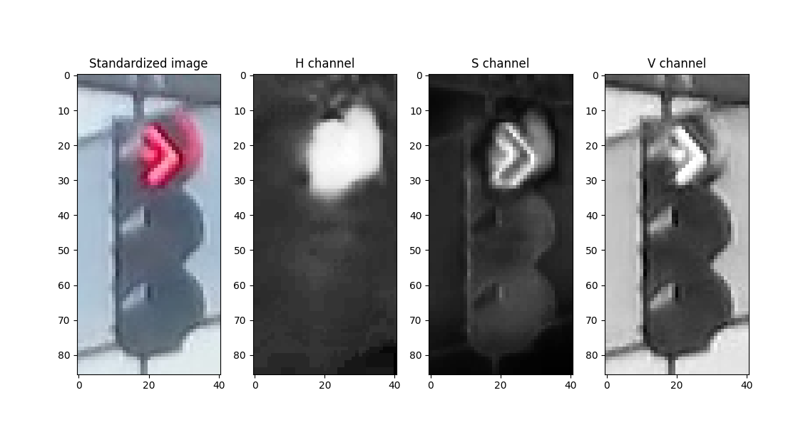
HSV色彩模型简介
常用的 RGB 色彩模型适合于显示系统,但颜色的改变会同时引起全部三个分量的变化,并不利于对颜色进行对比。而 HSV 色彩模型更接近于人类对彩色的感知经验,非常直观地表达颜色的色调、鲜艳程度与明暗程度,方便进行颜色的对比。
HSV 通过三个部分表示彩色图像:
- Hue - 色调、色相
- Saturation - 饱和度
- Value - 明度

以此圆柱体表示 HSV,圆柱体的横截面可以视为一个极坐标系,极坐标的极角表示 H,极轴长度表示 S,垂直于极坐标平面的高度方向则表示 V。不同的色相 H 表示不同的颜色,从 Hue=0° 表示红色开始,逆时针旋转一周,Hue=120° 表示绿色、Hue=240°表示蓝色等。以某个特定的 H 值,取圆柱体的半边横截面得到的矩形,水平方向表示 Saturation 饱和度,竖直方向表示 Value 明度。饱和度越高,颜色越接近光谱色,颜色越深;饱和度越低,颜色越接近白色越浅。明度越高,则颜色越明亮。
算法设计思想
有了 HSV 色彩模型,便容易实现交通信号灯图像识别分类了:色相通道可以独立地指定颜色;饱和度通道不受光照条件的影响,可以较好地识别对象边界。
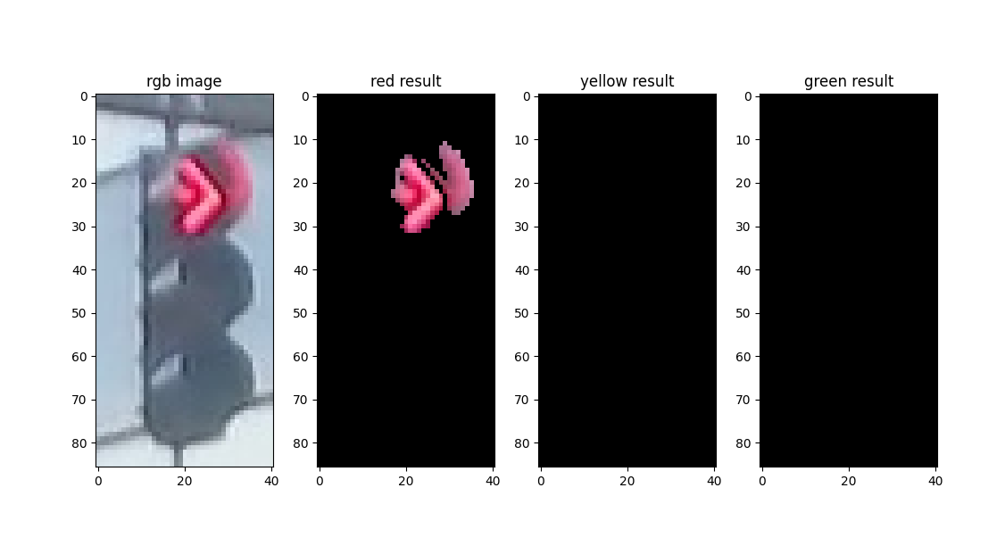
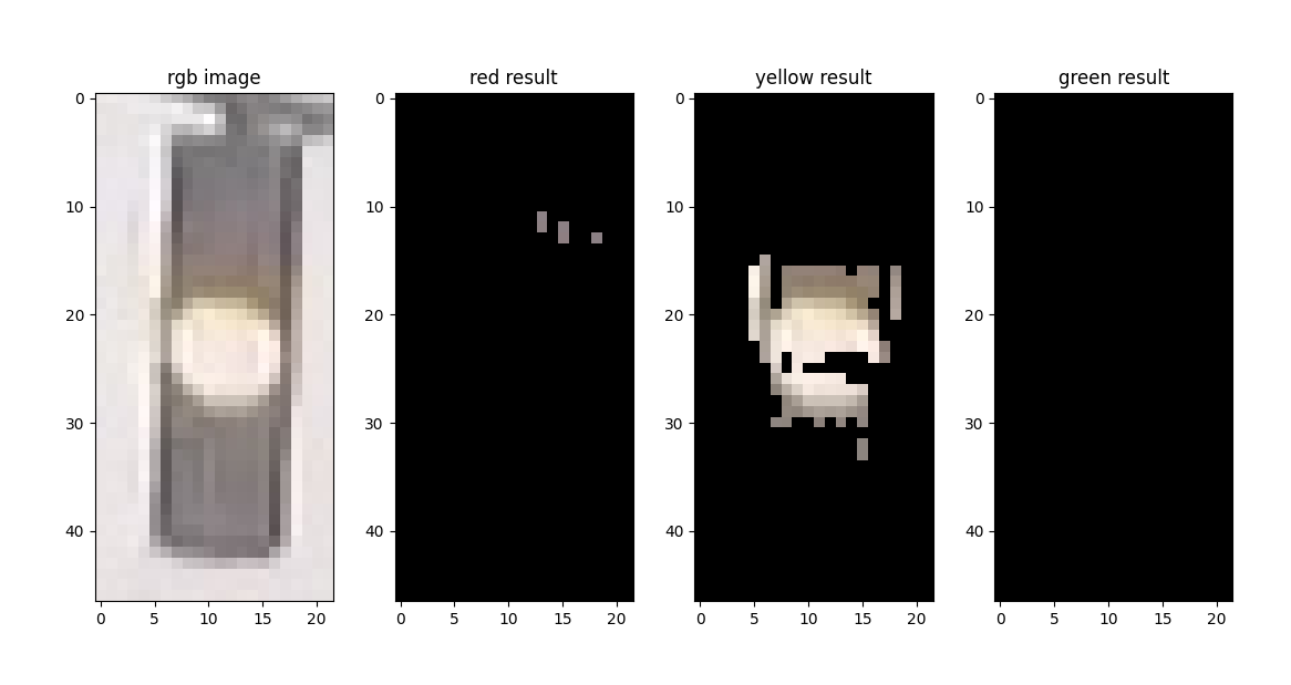
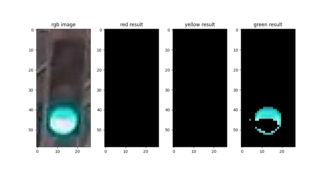
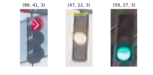
对于交通信号灯图片,灯光部分的饱和度明显高于其他部分,有明显的对象边界。因此可以设计计算饱和度阈值,将低于该阈值的像素全部抹去,实现提取灯光部分的效果。
再加上特定颜色(红、黄、绿)、适当的明度范围,即可获得适用于该张图像的掩膜(mask)。经掩膜处理后,若图像的剩余部分仍有大量非空像素(图中非黑色部分),则可以判断为对应颜色的信号灯。
代码实现
本文介绍的算法相关代码已经全部开源至Github - muziing/Traffic-Lights-Classification。
安装与导入第三方包
使用的所有第三方包列表及详细版本信息可以参考代码仓库中的 requirements.txt 或 poetry.lock 文件。
1 | |
加载数据与添加标签
数据集来源已不可考,据称来自于MIT自动驾驶课程,包含1187张交通信号灯图像,其中有723张红灯、35张黄灯与429张绿灯。注意本文并未使用机器学习方法,而直接以原数据集中的训练集作为编写、调试、测试算法性能的全集。
首先定义分类标签,使用枚举值类型,包含红、黄、绿三种颜色与未识别。
1 | |
编写代码,遍历所有图像文件,读取图像数据,与其颜色标签构成二元元组,一起保存至列表中备用。
1 | |
图像标准化处理
由于原始图像像素尺寸不一,可以考虑添加标准化代码,使其尺寸统一。将太大的图像缩小也有利于提高速度。
经实验,直接使用原始图像进行处理耗时24秒、识别错误20张图像;标注化至32*64像素,耗时20秒、识别错误20张图像;标准化至32*32像素,耗时10秒、识别错误21张图像;标准化至16*32像素,耗时5秒、识别错误24张图像。标准化图像尺寸(缩小)可以在精度牺牲很小的前提下明显提升运行速度,有一定意义。
1 | |
HSV空间下的图像处理
get_avg_saturation() 函数用于计算图像中所有像素的平均饱和度,未来将以此为依据,设定 S 通道掩码的下界。而 apply_mask() 函数则为指定的颜色(范围)创建掩膜,并应用于原始图像。
1 | |
算法主函数
算法参数设定如下:
1 | |
算法主函数:
1 | |
运行测试
最后编写测试函数,将测试图片逐张传入算法函数,获得对应的预测标签,再与实际标签比对,得知算法是否准确。
1 | |
经测试,1187张图像中仅有21张分类错误,准确度为98.23%。
可视化绘图
还编写了数个可视化绘图函数,便于直观检查算法运行情况。
1 | |
总结
使用 OpenCV 进行图像处理,将图像转至 HSV 色彩空间,运用适当的掩膜提取出关注部分,比较关注部分非空像素值的个数,最终实现了交通信号灯识别分类算法。该算法实现简单,运算速度快,经简单调参后可以达到98%以上的正确率,效果较好。